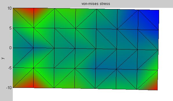
3年前学习Matlab时写的一段简单的有限元程序,使用三角形平面应力单元,模拟一块左边固定,右下角受拉的薄板的位移和应力分布情况。所有的前处理、刚度矩阵和外力矩阵的组装,以及求解和后处理均在程序内部完成。当时求解结果和ANSYS 做过比对,基本完全一致。
Matlab 版本的Von Mises 应力云图(变形500倍放大):
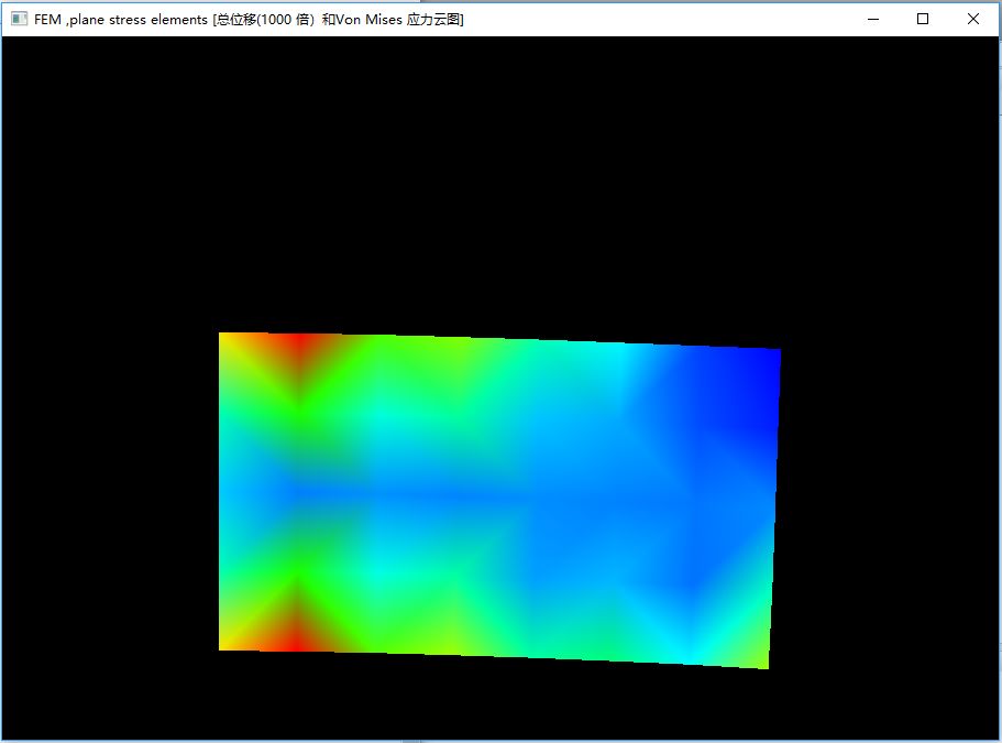
现已用python改写,初步完成。位移基本一致。由于精度问题,以及由于应力是变形的二次计算结果,所以应力分布略有不同。以后有空的话会继续完善。
python版本的Von Mises 应力云图(变形1000倍放大):
代码如下:
from numpy import * from numpy.linalg import det, solve#由几年前写的matlab代码翻译而来,author:wang_sp
注意matlab矩阵索引都是从1开始,而python、numpy索引都是从0 开始
#还有其它诸多不同
#单位体系 N,mm, ton#前处理
材料 material: ID,TYEP ,parameters(eg. E,nuxy,dens...)
MAT=mat([[1,1], [2,2]])
材料属性 materaial parameters for type 1:matID, E,nuxy,dens
#碳钢和铝合金.
MatPrmt= mat([[1,200000,0.3,7.85E-9], [2,69000,0.31,2.75E-9]],dtype =double)
#单元 element properity: ID, TYPE
PRPT=mat([[1,1], [2,1]])
#element parameters for type 1:PRPT ID,t(thickness)
PrptPrmt=mat([[1,1.0], [2,0.5]])
#Nodes info.: ID,x,y,z. #Node Id must start from 1,the step is 1.
#40个节点的简单FEM 模型
NODE= mat([[1,0,-10,0],
[2,0, -5,0],
[3,0,0,0],
[4,0,5,0],
[5,0, 10,0],
[6,5,-10,0],
[7,5, -5,0],
[8,5,0,0],
[9,5,5,0],
[10,5,10,0],
[11,10,-10,0],
[12,10, -5,0],
[13,10,0,0],
[14,10,5,0],
[15,10, 10,0],
[16,15,-10,0],
[17,15, -5,0],
[18,15,0,0],
[19,15,5,0],
[20,15, 10,0],
[21,20,-10,0],
[22,20, -5,0],
[23,20,0,0],
[24,20,5,0],
[25,20, 10,0],
[26,25,-10,0],
[27,25, -5,0],
[28,25,0,0],
[29,25,5,0],
[30,25, 10,0],
[31,30,-10,0],
[32,30, -5,0],
[33,30,0,0],
[34,30,5,0],
[35,30, 10,0],
[36,35,-10,0],
[37,35, -5,0],
[38,35,0,0],
[39,35,5,0],
[40,35, 10,0]],
dtype=double)
node_num = NODE.shape[0] #节点数量,40
#Element ID,MAT ID,TYPE ID,3 Nodes' ID
#56个平面应力单元
ELEM=mat([[1,1,1,1,6,7],
[2,1,1,1,7,2],
[3,1,1,2,7,8],
[4,1,1,2,8,3],
[5,1,1,3,8,4],
[6,1,1,4,8,9],
[7,1,1,4,9,5],
[8,1,1,5,9,10],
[9,1,1,6,11,7],
[10,1,1,7,11,12],
[11,1,1,7,12,13],
[12,1,1,7,13,8],
[13,1,1,8,13,9],
[14,1,1,9,13,14],
[15,1,1,9,14,15],
[16,1,1,9,15,10],
[17,1,1,11,16,17],
[18,1,1,11,17,12],
[19,1,1,12,17,18],
[20,1,1,12,18,13],
[21,1,1,13,18,14],
[22,1,1,14,18,19],
[23,1,1,14,19,15],
[24,1,1,15,19,20],
[25,1,1,16,21,17],
[26,1,1,17,21,22],
[27,1,1,17,22,23],
[28,1,1,17,23,18],
[29,1,1,18,23,19],
[30,1,1,19,23,24],
[31,1,1,19,24,25],
[32,1,1,19,25,20],
[33,1,1,21,26,27],
[34,1,1,21,27,22],
[35,1,1,22,27,28],
[36,1,1,22,28,23],
[37,1,1,23,28,24],
[38,1,1,24,28,29],
[39,1,1,24,29,25],
[40,1,1,25,29,30],
[41,1,1,26,31,27],
[42,1,1,27,31,32],
[43,1,1,27,32,33],
[44,1,1,27,33,28],
[45,1,1,28,33,29],
[46,1,1,29,33,34],
[47,1,1,29,34,35],
[48,1,1,29,35,30],
[49,1,1,31,36,37],
[50,1,1,31,37,32],
[51,1,1,32,37,38],
[52,1,1,32,38,33],
[53,1,1,33,38,34],
[54,1,1,34,38,39],
[55,1,1,34,39,35],
[56,1,1,35,39,40]],
dtype=integer)
elem_num = ELEM.shape[0] #单元数量,56
#Boundary conditions
#外力 Force矩阵
F = mat(zeros((node_num*2,1)), dtype=double)
'''
%F=spalloc(node_num*2,1,node_num*2);
%F(2*(5-1)+2)=10; % Fy on node 5
%F(2*(6-1)+1)=0; % Fx on node 6
%F(2*(6-1)+2)=10; % Fy on node 6
'''
F[2*(36-1)+1]=-10 # Fy on node 36,向下 10N#节点自由度 dof constrain
#node id, dof id(1 for x,2 for y...),dof value
CONS=mat([[1,1,0],
[1,2,0],
[2,1,0],
[2,2,0],
[3,1,0],
[3,2,0],
[4,1,0],
[4,2,0],
[5,1,0],
[5,2,0]])#生成有限元(FEM) 数学模型:
#K=spalloc(node_num2,node_num2,node_num*2) #matlab%(total nodes num. x dofs_per_node)'''
K= mat(zeros((node_num*2,node_num*2)), dtype=double)#初始化总刚度矩阵
B = zeros((elem_num,3,6), dtype=double) # 单元应变矩阵 ,全部单元的都存到数组
#各个单元的节点坐标
X=mat(zeros((3,elem_num)), dtype=double)
Y=mat(zeros((3,elem_num)),dtype=double)
#遍历单元
for ii in range(elem_num):
#材料属性
if ELEM[ii, 1] == 1: #to be updated
E = MatPrmt[0,1] #弹性模量
nuxy = MatPrmt[0,3] #泊松比
dens=MatPrmt[0,3] #密度
if ELEM[ii,2]==1: # to be updated
t = PrptPrmt[0,1] # thickness for plane stree elem
#弹性矩阵, 对称
D = E/(1-nuxy**2)* mat([[1,nuxy,0],[nuxy,1,0],[0,0,(1-nuxy)/2]])
#% nodes contained in the current element.单元的三个节点:
i = ELEM[ii,3]# Node ID
j = ELEM[ii,4]# Node ID
m = ELEM[ii,5]# Node ID#for jj=1:node_num #遍历节点,找出单元对应3个节点 # coordiates of the nodes contained in the current element flagi=0 flagj=0 flagm=0 for jj in range(node_num): if NODE[jj,0]==i: xi=NODE[jj,1] yi=NODE[jj,2] #zi=NODE[jj,3] flagi=1 continue elif NODE[jj,0]==j: xj=NODE[jj,1] yj=NODE[jj,2] # zj=NODE[jj,3] flagj=1 continue elif NODE[jj,0]==m: xm=NODE[jj,1] ym=NODE[jj,2] #zm=NODE[jj,3] flagm=1 continue else: pass if flagi*flagj*flagm==1: break X[: ,ii ] = mat([[xi], [xj], [xm]])#X坐标 Y[: ,ii ] = mat([[yi], [yj], [ym]])#Y坐标 A=0.5*det(mat([[1,xi,yi],[1,xj,yj],[1,xm,ym]]))# 三角形(单元)的面积( Area for triangle) #单元应变矩阵Be=[Bi,Bj,Bm] Bi=mat([[yj-ym,0], [0,-xj+xm], [-xj+xm,yj-ym]])/(2*A) Bj=mat([[ym-yi,0], [0,-xm+xi], [-xm+xi,ym-yi]])/(2*A) Bm=mat([[yi-yj,0], [0,-xi+xj], [-xi+xj,yi-yj]])/(2*A) #分块矩阵组装 B[ii] = bmat("Bi Bj Bm")#仍是数组 #单元刚度矩阵Ke=[Kii,Kij,Kim;Kji,Kjj,Kjm;Kmi,Kmj,Kmm] #更新总刚度矩阵 Kii = Bi.T * D * Bi *A*t #K(2*i-1:2*i,2*i-1:2*i)=K(2*i-1:2*i,2*i-1:2*i)+Kii;%matlab 包含冒号后面那个,numpy不含 K[2*i-2 : 2*i , 2*i-2 : 2*i] += Kii Kij=Bi.T * D * Bj * A * t #K(2*i-1:2*i,2*j-1:2*j)=K(2*i-1:2*i,2*j-1:2*j)+Kij; K[2*i-2 : 2*i, 2*j-2 : 2*j] += Kij Kim=Bi.T* D * Bm * A * t # K(2*i-1:2*i,2*m-1:2*m)=K(2*i-1:2*i,2*m-1:2*m)+Kim; K[2*i -2 : 2*i, 2*m-2: 2*m] += Kim Kji=Bj.T*D*Bi*A*t # K(2*j-1:2*j,2*i-1:2*i)=K(2*j-1:2*j,2*i-1:2*i)+Kji; K[2*j-2 :2*j, 2*i-2: 2*i] += Kji Kjj=Bj.T*D*Bj*A*t # K(2*j-1:2*j,2*j-1:2*j)=K(2*j-1:2*j,2*j-1:2*j)+Kjj; K[2*j - 2 : 2*j, 2*j -2: 2*j] += Kjj Kjm=Bj.T*D*Bm*A*t # K(2*j-1:2*j,2*m-1:2*m)=K(2*j-1:2*j,2*m-1:2*m)+Kjm; K[2*j-2: 2*j, 2*m -2: 2*m] += Kjm Kmi=Bm.T*D*Bi*A*t # K(2*m-1:2*m,2*i-1:2*i)=K(2*m-1:2*m,2*i-1:2*i)+Kmi; K[2*m-2 : 2*m, 2*i -2 : 2*i] += Kmi Kmj=Bm.T*D*Bj*A*t # K(2*m-1:2*m,2*j-1:2*j)=K(2*m-1:2*m,2*j-1:2*j)+Kmj; K[2*m-2:2*m,2*j-2:2*j] += Kmj Kmm=Bm.T*D*Bm*A*t # K(2*m-1:2*m,2*m-1:2*m)=K(2*m-1:2*m,2*m-1:2*m)+Kmm; K[2*m-2:2*m,2*m-2:2*m] += Kmm;#% Kff updated from K as per Boundary conditions
#将边界条件(力,位移约束)更新到刚度矩阵;更新外力矩阵
Kff=K[:,:]
BigNum = 1.0e150#大数法
cr = CONS.shape[0]
#遍历约束节点
for ii in range(cr):
jj = 2*(CONS[ii,0]-1)+CONS[ii,1]
Kff[jj-1, jj-1] *= BigNum
F[jj-1] = CONS[ii-1, 2]*Kff[jj-1, jj-1]*BigNumSOLVE
求解 位移矩阵Deformation Matrix Delta
Delta= solve(Kff, F)#位移矩阵
#Delta value from solve replaced by the iputed constrain value
#even though there is nearly no difference
#遍历节点,尽管几乎没有差别(计算精度问题)
#还是将位移在边界节点上的值用输入的约束值修正
for ii in range(cr):
jj = 2*(CONS[ii,0]-1)+CONS[ii,1]
Delta[jj-1] = CONS[ii,2]
print("位移矩阵:"); print(Delta)#后处理
#应变矩阵
Epsilon = mat(zeros((4,node_num)),dtype=double)#% used to store node strain(sum at the current loop)
#应力矩阵
Sigma=mat(zeros((3,node_num)),dtype=double)#% used to store node stress(sum at the current loop)
cnte = mat(zeros((1,node_num)),dtype=integer)# %count of elements surrouding each node
#遍历单元
for ii in range(elem_num):
#材料属性
if ELEM[ii, 1] == 1: #to be updated
E = MatPrmt[0,1] #弹性模量
nuxy = MatPrmt[0,3] #泊松比
dens=MatPrmt[0,3] #密度
if ELEM[ii,2]==1: # to be updated
t = PrptPrmt[0,1] # thickness for plane stree elem
#弹性矩阵, 对称
D = E/(1-nuxy**2)* mat([[1,nuxy,0],[nuxy,1,0],[0,0,(1-nuxy)/2]])
#% nodes contained in the current element.单元的三个节点:
i = ELEM[ii,3]# Node ID
j = ELEM[ii,4]# Node ID
m = ELEM[ii,5]# Node ID
#单元位移矩阵
#print(Delta[2*(i-1),0])
Delta_e=mat([[Delta[2*(i-1),0]],[Delta[2*(i-1)+1, 0]], [Delta[2*(j-1),0]],[Delta[2*(j-1)+1,0]],[Delta[2*(m-1),0]],[Delta[2*(m-1)+1,0]]])
#print(Delta_e)
#单元应变矩阵,ex,elem_num,rxy
Strain_e= mat(B[ii])*Delta_e; # without ez
#单元应力矩阵
Stress_e= D * Strain_e# 添加Z向应变,with ez(strain of z direction) Strain_e = mat([[Strain_e[0,0]], [Strain_e[1,0]], [Strain_e[2,0]] , [-nuxy/E*(Stress_e[0,0]+Stress_e[1,0])]]) #先求和,后面平均 Epsilon[:,i-1] += Strain_e Epsilon[:,j-1] += Strain_e Epsilon[:,m-1] += Strain_e Sigma[:,i-1] += Stress_e Sigma[:,j-1] += Stress_e Sigma[:,m-1] += Stress_e cnte[:,i-1] += 1 cnte[:,j-1] += 1 cnte[:,m-1] += 1#Epsilon=Epsilon./repmat(cnte,4,1)
Epsilon = Epsilon/ tile(cnte,(4,1))
Sigma = Sigma / tile(cnte,(3,1))
#之前位移矩阵内数的排列次序是节点1 x向位移,节点1 y向位移; 节点2....
#提高可读性:现在每个节点Ux,Uy 显示在同一行
Delta = Delta.reshape((-1,2))
print("位移矩阵(unit: mm):"); print(Delta)
Epsilon = Epsilon.T # x,y,xy,z 应变
Sigma = Sigma.T
#F=(reshape(F,2,node_num))';% more readable; Fx,Fy for one node listed on one row
#postprocesstotal Deformation 总位移
Delta_sum = sqrt(array(Delta[:, 0])**2 + array(Delta[:, 1])**2)
Sigma1 = (Sigma[:, 0] + Sigma[:,1])/2.0 + sqrt( array(Sigma[:, 0] - Sigma[:,1]/2.0)**2 +array(Sigma[:,2])**2)
Sigma2 = (Sigma[:, 0] + Sigma[:,1])/2.0 - sqrt( array(Sigma[:, 0] - Sigma[:,1]/2.0)**2 +array(Sigma[:,2])**2)
#冯米塞斯应力 Von Mises Stress #by Node
Sigma_eqv = sqrt(array(Sigma1)**2 + array(Sigma2)**2 + array(Sigma1 -Sigma2)**2/2.0)
print(Sigma_eqv.shape) #(40,1)
print(Sigma_eqv[1,0])X_delta = zeros((3,elem_num), dtype=double)
Y_delta = zeros((3,elem_num), dtype=double)
for ii in range(elem_num):
i = ELEM[ii,3]# Node ID
j = ELEM[ii,4]# Node ID
m = ELEM[ii,5]# Node ID
X_delta[:,ii] = Delta[[i-1 ,j-1 ,m-1],0].reshape(3) #for one element
Y_delta[:,ii] = Delta[[i-1 ,j-1 ,m-1],1].reshape(3) #for one element#结果可视化
scale = 1000 #变形量放大系数
X_new = X+scaleX_delta
Y_new = Y+scaleY_delta
def num2RGB(x,LSL=0, USL=1.0):
r=(x-LSL)/(USL-LSL)
if r>1:
return (1, 1, 1)
elif r>=0.75:
return (1, 1*(1-r)*4, 0)
elif r>=0.5:
return (1*(r-0.5)*4, 1, 0)
elif r>=0.25:
return (0, 1, 1*(0.5-r)*4)
elif r>=0:
return (0, 1*r*4, 1)
else:
return (0.0,0.0,0.0)import sys
from PyQt5.QtCore import *
from PyQt5.QtGui import *
from PyQt5.QtWidgets import *
from PyQt5.QtOpenGL import QGLWidget
from OpenGL import GL
class GLWidget(QGLWidget):
def init(self, parent =None):
super(GLWidget, self).init(parent)
def initializeGL(self):
self.qglClearColor(QColor("black")) #背景色
#GL.glClearDepth(1.0)# Enables Clearing Of The Depth Buffer
GL.glShadeModel(GL.GL_SMOOTH) #!颜色平滑渲染
#GL.glDepthFunc(GL.GL_LESS) # The Type Of Depth Test To Do
#GL.glEnable(GL.GL_DEPTH_TEST)
self.object = self.makeObject()def paintGL(self): GL.glClear(GL.GL_COLOR_BUFFER_BIT | GL.GL_DEPTH_BUFFER_BIT) GL.glLoadIdentity()# Reset The Projection Matrix #GL.glTranslatef(0, 0.0, 0)#平移 #GL.glRotated(0.5, 1.0, 0.0, 0.0)#旋转 GL.glCallList(self.object) def resizeGL(self, width, height): side = min(width, height) GL.glViewport((width - side) // 2, (height - side) // 2, side, side)#保持图形的长宽比 #GL.glViewport(50,50,500,500) GL.glMatrixMode(GL.GL_PROJECTION) GL.glLoadIdentity()# Reset The Projection Matrix #GL.glOrtho(-0.5, +0.5, +0.5, -0.5, 4.0, 15.0) GL.glMatrixMode(GL.GL_MODELVIEW) def makeObject(self): genList = GL.glGenLists(1) GL.glNewList(genList, GL.GL_COMPILE) #位移和应力的可视化 global X_new, Y_new,elem_num, ELEM, Sigma_eqv XnewMin = X_new.min() YnewMin = Y_new.min() XnewMax = X_new.max() YnewMax = Y_new.max() L = -0.8 ; R = 0.8 RL = R-L #stress stressMin = Sigma_eqv.min() stressMax = Sigma_eqv.max() if XnewMax - XnewMin >= YnewMax - YnewMin:# X方向模型总长度更长(else则写法类似,暂略过) Span = XnewMax - XnewMin for i in range(elem_num): # Draw a 2d element GL.glBegin(GL.GL_POLYGON)# Start drawing a polygon for j in range(3): #For colors nodeID = int(ELEM[i,3+j]) #print(nodeID) stress = Sigma_eqv[nodeID-1, 0] # Node ID 从1开始,但是索引从0开始 #print(Sigma_eqv[1, 0]) r,g,b = num2RGB(stress, stressMin,stressMax) GL.glColor3f(r, g, b) x = (X_new[j,i] - XnewMin) /Span *RL + L y = (Y_new[j,i] - YnewMin) /Span *RL + L GL.glVertex2f(x, y) GL.glEnd() GL.glEndList() return genList def minimumSizeHint(self): return QSize(100, 100) #def sizeHint(self): #return QSize(800, 800)class MainWindow(QMainWindow):
def init(self):
super().init()
print("oo")
self.setCentralWidget(GLWidget())
global scale
self.setWindowTitle("FEM ,plane stress elements [总位移(%d 倍)和Von Mises 应力云图]" % scale )
self.resize(800, 800)
if name == 'main':
app = QApplication(sys.argv)
mainWin = MainWindow()
mainWin.show()
sys.exit(app.exec_())