ClassificationExample.m
%% ================== Generate and Plot Training Set ================== %% clear all; close all; clc;n = 2; % number of feature dimensions
N = 1000; % number of iid samples% parallel distributions
mu(:,1) = [2;0]; Sigma(:,:,2) = [2 0.5;0.5 30];
mu(:,2) = [-2;0]; Sigma(:,:,1) = [2 0.5;0.5 30];
%mu(:,1) = [3;0]; Sigma(:,:,1) = [5 0.1;0.1 .5];
%mu(:,2) = [0;0]; Sigma(:,:,2) = [.5 0.1;0.1 5];% Class priors for class 0 and 1 respectively
p = [0.5,0.5];% Generating true class labels
label = (rand(1,N) >= p(1))';
Nc = [length(find(label==0)),length(find(label==1))];% Draw samples from each class pdf
x = zeros(N,n);
for L = 0:1
x(label==L,:) = mvnrnd(mu(:,L+1),Sigma(:,:,L+1),Nc(L+1));
end%Plot samples with true class labels
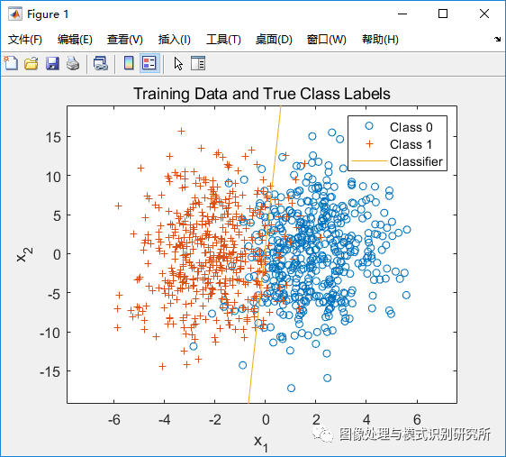
figure(1);
plot(x(label==0,1),x(label==0,2),'o',x(label==1,1),x(label==1,2),'+');
legend('Class 0','Class 1'); title('Training Data and True Class Labels');
xlabel('x_1'); ylabel('x_2'); hold on;%% ======================== Logistic Regression ======================= %%
% Initialize fitting parameters
x = [ones(N, 1) x];
initial_theta = zeros(n+1, 1);
label=double(label);% Compute gradient descent to get theta values
[theta, cost] = fminsearch(@(t)(cost_func(t, x, label, N)), initial_theta);% Choose points to draw boundary line
plot_x1 = [min(x(:,2))-2, max(x(:,2))+2];
plot_x2 = (-1./theta(3)).*(theta(2).*plot_x1 + theta(1));% Plot decision boundary
plot(plot_x1, plot_x2);
axis([plot_x1(1), plot_x1(2), min(x(:,3))-2, max(x(:,3))+2]);
legend('Class 0', 'Class 1', 'Classifier');%% ====================== Generate Test Data Set ====================== %%
N_test = 10000;% Generating true class labels
label_test = (rand(1,N_test) >= p(1))';
Nc_test = [length(find(label_test==0)),length(find(label_test==1))];% Draw samples from each class pdf
x_test = zeros(N_test,n);
for L = 0:1
x_test(label_test==L,:) = mvnrnd(mu(:,L+1),Sigma(:,:,L+1),Nc_test(L+1));
end%% ========================= Test Classifier ========================== %%
% % Coefficients for decision boundary line equation
% coeff = polyfit([plot_x1(1), plot_x1(2)], [plot_x2(1), plot_x2(2)], 1);
% % Decide based on which side of the line each point is on
% if coeff(1) >= 0
% decision = (coeff(1).*x_test(:,1) + coeff(2)) < x_test(:,2);
% else
% decision = (coeff(1).*x_test(:,1) + coeff(2)) > x_test(:,2);
% endtesty = [ones(N_test, 1) x_test];
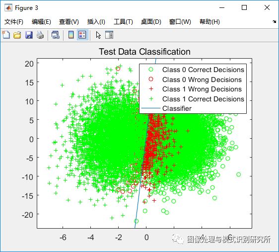
decision = testy*theta >= 0;%plot_results(decision(:,1),label_test,Nc_test,3,x_test,plot_x1,plot_x2(1,:),p);
% Count correct and incorrect decisions
ind00 = find(decision==0 & label_test==0); % true negative
ind10 = find(decision==1 & label_test==0); p10 = length(ind10)/Nc_test(1); % false positive
ind01 = find(decision==0 & label_test==1); p01 = length(ind01)/Nc_test(2); % false negative
ind11 = find(decision==1 & label_test==1); % true positive
fprintf('Total error with 10,000 test points: %.2f%%\n',(p10*p(1) + p01*p(2))*100);% Plot decisions and decision boundary
figure(3);
plot(x_test(ind00,1),x_test(ind00,2),'og'); hold on,
plot(x_test(ind10,1),x_test(ind10,2),'or'); hold on,
plot(x_test(ind01,1),x_test(ind01,2),'+r'); hold on,
plot(x_test(ind11,1),x_test(ind11,2),'+g'); hold on,
plot(plot_x1, plot_x2(1,:));
axis([plot_x1(1), plot_x1(2), min(x_test(:,2))-2, max(x_test(:,2))+2])
title('Test Data Classification');
legend('Class 0 Correct Decisions','Class 0 Wrong Decisions','Class 1 Wrong Decisions','Class 1 Correct Decisions','Classifier');%% ============================ Functions ============================= %%
function [theta, cost] = gradient_descent(x, N, label, theta, alpha, num_iters)
cost = zeros(num_iters, 1);
for i = 1:num_iters
h = 1 ./ (1 + exp(-xtheta)); % Sigmoid function
cost(i) = (-1/N)((sum(label' * log(h)))+(sum((1-label)' * log(1-h))));
cost_gradient = (1/N)*(x' * (h - label));
theta = theta - (alpha.*cost_gradient); % Update theta
end
end
function cost = cost_func(theta, x, label,N)
h = 1 ./ (1 + exp(-xtheta)); % Sigmoid function
cost = (-1/N)((sum(label' * log(h)))+(sum((1-label)' * log(1-h))));
end
Deric_ClassExample2v2.m
%% ================== Generate and Plot Training Set ================== %%
clear all; close all; clc;n = 2; % number of feature dimensions
N = 1000; % number of iid samples% parallel distributions
mu(:,1) = [2;0]; Sigma(:,:,2) = [2 0.5;0.5 30];
mu(:,2) = [-2;0]; Sigma(:,:,1) = [2 0.5;0.5 30];
%mu(:,1) = [3;0]; Sigma(:,:,1) = [5 0.1;0.1 .5];
%mu(:,2) = [0;0]; Sigma(:,:,2) = [.5 0.1;0.1 5];% Class priors for class 0 and 1 respectively
p = [0.5,0.5];% Generating true class labels
label = (rand(1,N) >= p(1))';
Nc = [length(find(label==0)),length(find(label==1))];% Draw samples from each class pdf
x = zeros(N,n);
for L = 0:1
x(label==L,:) = mvnrnd(mu(:,L+1),Sigma(:,:,L+1),Nc(L+1));
end%Plot samples with true class labels
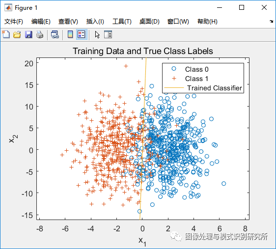
figure(1);
plot(x(label==0,1),x(label==0,2),'o',x(label==1,1),x(label==1,2),'+');
legend('Class 0','Class 1'); title('Training Data and True Class Labels');
xlabel('x_1'); ylabel('x_2'); hold on;%% ======================== Computing Gradient ======================== %%
% Initialize fitting parameters
x = [ones(N, 1) x];
initial_theta = zeros(n+1, 1);
label=double(label);% Compute gradient descent to get theta values
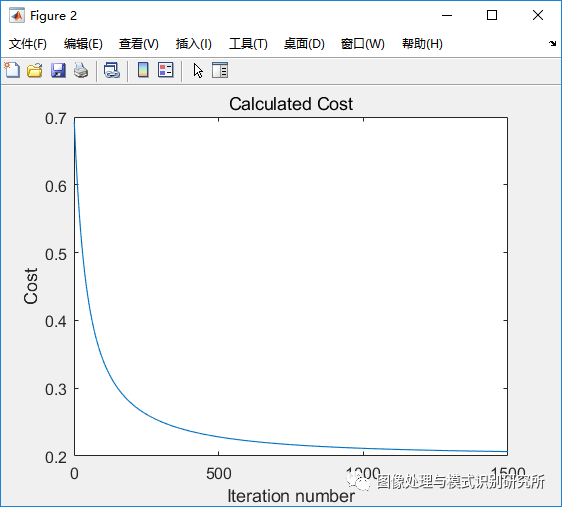
[theta, cost] = gradientDescent(x,N,label,initial_theta,0.01,1500);% Choose points to draw boundary line
plot_x1 = [min(x(:,2))-2, max(x(:,2))+2]; % x1 value
plot_x2 = (-1./theta(3)).*(theta(2).*plot_x1 + theta(1)); % corresponding x2% Plot decision boundary
plot(plot_x1, plot_x2);
axis([plot_x1(1), plot_x1(2), min(x(:,3))-2, max(x(:,3))+2]);
legend('Class 0', 'Class 1', ' Trained Classifier');% Plot cost function
figure(2); plot(cost);
title('Calculated Cost');
xlabel('Iteration number'); ylabel('Cost');%%
[theta, cost] = fmisearch(@(t) costFunction(t,x,label,N), initial_theta);%% ====================== Generate Test Data Set ====================== %%
N_test = 10000;% Generating true class labels
label_test = (rand(1,N_test) >= p(1))';
Nc_test = [length(find(label_test==0)),length(find(label_test==1))];% Draw samples from each class pdf
x_test = zeros(N_test,n);
for L = 0:1
x_test(label_test==L,:) = mvnrnd(mu(:,L+1),Sigma(:,:,L+1),Nc_test(L+1));
end%% ========================= Test Classifier ========================== %%
% Coefficients for decision boundary line equation
coeff = polyfit([plot_x1(1), plot_x1(2)], [plot_x2(1), plot_x2(2)], 1);
% Decide based on which side of the line each point is on
if coeff(1) >= 0
decision = (coeff(1).*x_test(:,1) + coeff(2)) < x_test(:,2);
else
decision = (coeff(1).*x_test(:,1) + coeff(2)) > x_test(:,2);
end% Count correct and incorrect decisions
ind00 = find(decision==0 & label_test==0); % true negative
ind10 = find(decision==1 & label_test==0); p10 = length(ind10)/Nc_test(1); % false positive
ind01 = find(decision==0 & label_test==1); p01 = length(ind01)/Nc_test(2); % false negative
ind11 = find(decision==1 & label_test==1); % true positive
fprintf('Total error with 10,000 test points: %.2f%%\n',(p10*p(1) + p01*p(2))*100);% Plot decisions and decision boundary
figure(3);
plot(x_test(ind00,1),x_test(ind00,2),'og'); hold on,
plot(x_test(ind10,1),x_test(ind10,2),'or'); hold on,
plot(x_test(ind01,1),x_test(ind01,2),'+r'); hold on,
plot(x_test(ind11,1),x_test(ind11,2),'+g'); hold on,
plot(plot_x1, plot_x2);
axis([plot_x1(1), plot_x1(2), min(x(:,3))-2, max(x(:,3))+2])
title('Test Data Classification');
legend('Class 0 Correct Decisions','Class 0 Wrong Decisions','Class 1 Wrong Decisions','Class 1 Correct Decisions','Classifier');
%% ==================== Gradient Descent Function ==================== %%
function [theta, cost] = gradientDescent(x, N, label, theta, alpha, num_iters)
cost = zeros(num_iters, 1);
for i = 1:num_iters
h = 1 ./ (1 + exp(-xtheta)); % Sigmoid function
cost(i) = (-1/N)((sum(label' * log(h)))+(sum((1-label)' * log(1-h))));
cost_gradient = (1/N)(x' * (h - label));
theta = theta - (alpha.cost_gradient);
end
end
%%
function J = costFunction(theta, x, label,N)
h = 1 ./ (1 + exp(-xtheta));
J = (-1/N)((sum(label' * log(h)))+(sum((1-label)' * log(1-h))));
end
evalGaussian.m
function g = evalGaussian(x,mu,Sigma)
% Evaluates the Gaussian pdf N(mu,Sigma) at each coumn of X
[n,N] = size(x);C = ((2pi)^n * det(Sigma))^(-1/2); % coefficient
E = -0.5sum((x-repmat(mu,1,N)).(inv(Sigma)(x-repmat(mu,1,N))),1); % exponent
g = C*exp(E); % final gaussian evaluation
end