Jupyter Notebook 是一个开源的 Web 应用程序,可以用来创建和共享包含动态代码、方程式、可视化及解释性文本的文档。其应用于包括:数据整理与转换,数值模拟,统计建模,机器学习等等。
安装 Jupyter Notebook
Jupyter Notebook 简介
Jupyter Notebook 是一个开源的 Web 应用程序,可以用来创建和共享包含动态代码、方程式、可视化及解释性文本的文档。
其应用于包括:数据整理与转换,数值模拟,统计建模,机器学习等等。
更多信息请见 官网 。
检查 Python 环境
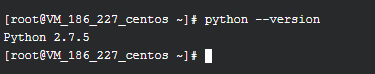
CentOS 7.2 中默认集成了 Python 2.7,可以通过下面命令检查 Python 版本:
python --version
安装 pip
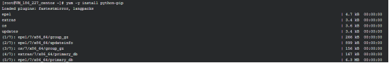
pip 是一个 Python 包管理工具,我们使用 yum 命令来安装该工具:
yum -y install python-pip
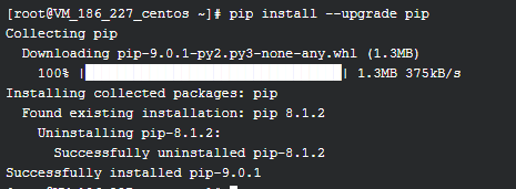
使用下面命令升级 pip 到最新版本:
pip install --upgrade pip
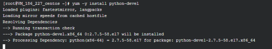
安装相关依赖
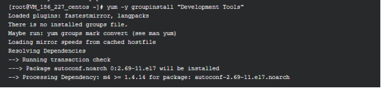
安装 Jupyter 过程中还需要其他一些依赖,我们使用以下命令安装他们:
yum -y groupinstall "Development Tools"
yum -y install python-devel
配置虚拟环境
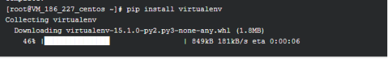
安装 virtualenv
我们将为 Jupyter 创建一个独立的虚拟环境,与系统自带的 Python 隔离开来。为此,先安装 virtualenv 库:
pip install virtualenv
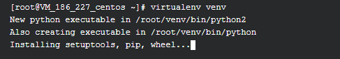
创建虚拟环境
创建一个专门的虚拟环境,并直接激活进入该环境:
virtualenv venv
source venv/bin/activate

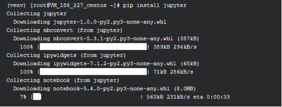
使用 pip 安装 Jupyter
我们使用 pip 命令安装 Jupyter:
pip install jupyter
配置 Jupyter Notebook
建立项目目录
我们先为 Jupyter 相关文件准备一个目录:
mkdir /data/jupyter
cd /data/jupyter
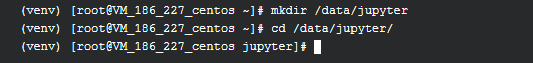
再建立一个目录作为 Jupyter 运行的根目录:
mkdir /data/jupyter/root

准备密码密文
由于我们将以需要密码验证的模式启动 Jupyter,所以我们要预先生成所需的密码对应的密文。
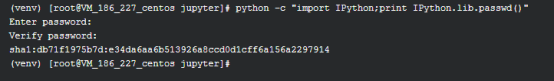
生成密文
使用下面的命令,创建一个密文的密码:
python -c "import IPython;print IPython.lib.passwd()"
执行后需要输入并确认密码,然后程序会返回一个 'sha1:...' 的密文,我们接下来将会用到它。

以123为例
修改配置
生成配置文件
我们使用 --generate-config 来参数生成默认配置文件:
jupyter notebook --generate-config --allow-root

生成的配置文件在 /root/.jupyter/ 目录下
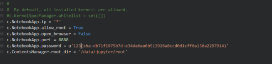
然后在配置文件最下方加入以下配置:
c.NotebookApp.ip = '*'
c.NotebookApp.allow_root = True
c.NotebookApp.open_browser = False
c.NotebookApp.port = 8888
c.NotebookApp.password = u'刚才生成的密文(sha:...)'
c.ContentsManager.root_dir = '/data/jupyter/root'
注意:如果浏览器出现验证失败Invalid credentials,请检查passwd这行
正确格式为:
c.NotebookApp.password = u'sha1:67c9e60bb8b6:9ffede0825894254b2e042ea597d771089e11aed'
如果出现报错99 尝试释放端口,或重启主机。修改上述passwd位置
其中:
c.NotebookApp.password 请将上一步中密文填入此项,包括 sha: 部分。
你也可以直接配置或使用 Nginx 将服务代理到 80 或 443 端口。
启动 Jupyter Notebook
直接启动
使用以下指令启动 Jupyter Notebook:
jupyter notebook
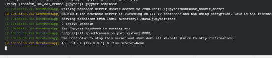
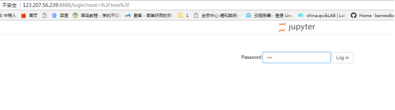
此时,访问 http://123.207.56.239:8888 即可进入 Jupyter 首页。
若出现上述页面,检查sha1的值
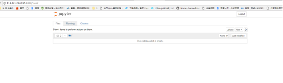
正常应显示如下:
创建 Notebook
进入【首页】首先需要输入前面步骤中设置的密码。
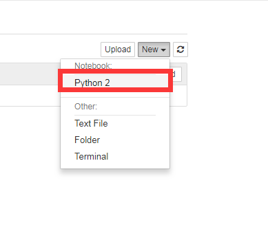
然后点击右侧的【 new 】,选择 Python2 新建一个 notebook,这时跳转至编辑界面。
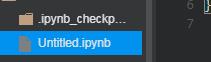
现在我们可以看到 /data/jupyter/root/ 目录中出现了一个 Untitled.ipynb 文件,这就是我们刚刚新建的 Notebook 文件。我们建立的所有 Notebook 都将默认以该类型的文件格式保存。
后台运行
直接以 jupyter notebook 命令启动 Jupyter 的方式在连接断开时将会中断,所以我们需要让 Jupyter 服务在后台常驻。
先按下 Ctrl + C 并输入 y 停止 Jupyter 服务,然后执行以下命令:
nohup jupyter notebook > /data/jupyter/jupyter.log 2>&1 &

该命令将使得 Jupyter 在后台运行,并将日志写在 /data/jupyter/jupyter.log 文件中。
准备后续步骤的 Notebook
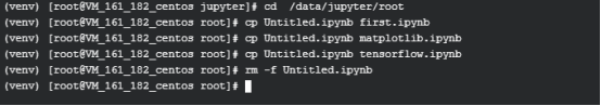
为了后面实验中实验室的步骤检查器能够更好的工作,此时我们使用以下命令预先创建几份 ipynb 文件:
cd /data/jupyter/root
cp Untitled.ipynb first.ipynb
cp Untitled.ipynb matplotlib.ipynb
cp Untitled.ipynb tensorflow.ipynb
rm -f Untitled.ipynb
使用 Jupyter Notebook
编辑界面
点击这里打开 first.ipynb 编辑界面。
Jupyter Notebook 的编辑界面主要由 工具栏 和 内容编辑区 构成。
下方编辑区,由 Cell 组成。每个 notebook 由多个 Cell 构成,每个 Cell 都可以有不同的用途。
Code Cell
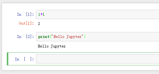
新建的 notebook 中包含一个代码 Cell(Code Cell),以 [ ] 开头,在该类型的 Cell 中,可以输入任意代码并执行。如输入:
1 + 1
然后按下 Shift + Enter 键, Cell 中代码就会被执行,光标也会移动至下个新 Cell 中。我们接着输入:
print('Hello Jupyter')
再次按下 Shift + Enter ,可以看到这次没有出现 Out[..] 这样的文字。这是因为我们只打印出来了某些值,而没有返回任何的值。
按下 Ctrl + S 保存
Heading Cell *
新版本中已经没有独立的 Heading Cell,现在标题被整合在 Markdown Cell 之中。
如果我们想在顶部添加一个的标题。选中第一个 Cell,然后点击 Insert -> Insert Cell Above。
你会发现,文档顶部马上就出现了一个新的 Cell。点击在工具栏中 Cell 类型(默认为 Code),将其变成 Markdown。接着在 Cell 中写下:
# My First Notebook
然后按下 Shift + Enter 键,便可以看到生成了一行一级标题。
与 Markdown 语法相同,使用多个#将改变标题级别。
Markdown Cell
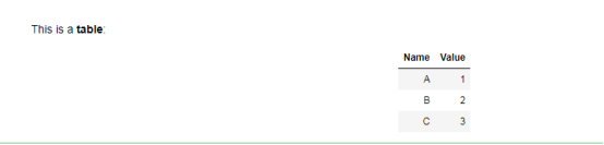
上一步中我们已经尝试了使用了 Markdown Cell。在该 Cell 中,除标题外其他语法同样支持。比如,我们在一个新的 Cell 中插入以下文本:
This is a **table**:
| Name | Value |
|:----:|:-----:|
| A | 1 |
| B | 2 |
| C | 3 |
然后按下 Shift + Enter,即可渲染出相应内容。
高级用法 - HTML
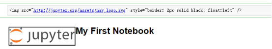
Markdown Cell 中同样接受 HTML 代码。这样,你就可以实现更加丰富的样式及结构、添加图片等等。
例如,如果想在 notebook 中添加 Jupyter 的 logo,并且添加 2px 的黑色边框,放置在单元格左侧,可以这样编写:
<img src="http://jupyter.org/assets/nav_logo.svg" style="border: 2px solid black; float:left" />
然后按下 Shift + Enter,即可渲染出图片。
高级用法 - LaTex
Markdown Cell 还支持 LaTex 语法。在 Cell 中插入以下文本:
$$int_0^{+infty} x^2 dx$$
同样按下 Shift + Enter,即可渲染出公式。
导出
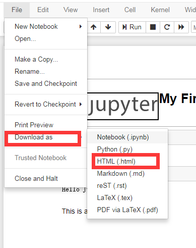
notebook 支持导出导出为 HTML、Markdown、PDF 等多种格式。
如点击 File -> Download as -> HTML(.html),即可下载到 HTML 版本的 notebook。
直接导出PDF 会报错,需要安装依赖
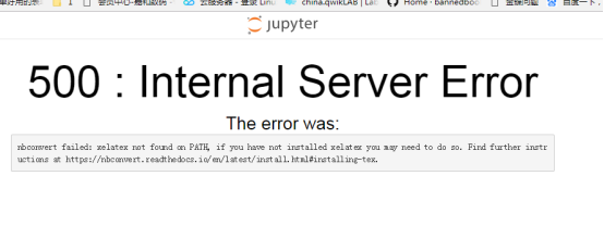
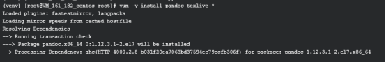
其中,导出 PDF 需要其他包的支持,我们需要使用以下命令安装这些依赖:
yum -y install pandoc texlive-*
注:直接导出 PDF 时 Jupyter 可能会忽略一些 Cell,建议先导出为 HTML,然后使用浏览器将其转为 PDF。
集成 Matplotlib(可选)
Matplotlib 是 Python 中最常用的可视化工具之一,可以非常方便地创建许多类型的 2D 图表和基本的 3D 图表。
安装 Matplotlib
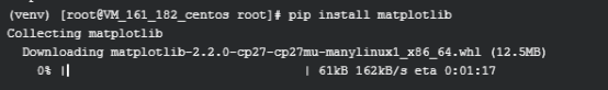
我们使用 pip 来安装 Matplotlib:
pip install matplotlib
测试 Matplotlib
我们使用另一个 notebook (matplotlib.ipynb)来测试 Matplotlib。
打开 matplotlib.ipynb 编辑界面。
魔法命令
在第一个 Cell 中,我们插入并执行:
%matplotlib inline
这是指定 matplotlib 图表的显示方式的魔法命令。inline 表示将图表嵌入到 notebook 中。
测试
关于 Matplotlib 的使用请移步其官网。
在接下来 Cell 中,我们插入几个官方示例测试:
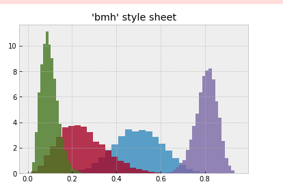
1.plot_bmh:
plot_bmh.py
from numpy.random import beta
import matplotlib.pyplot as plt
plt.style.use('bmh')
def plot_beta_hist(ax, a, b):
ax.hist(beta(a, b, size=10000), histtype="stepfilled",
bins=25, alpha=0.8, normed=True)
fig, ax = plt.subplots()
plot_beta_hist(ax, 10, 10)
plot_beta_hist(ax, 4, 12)
plot_beta_hist(ax, 50, 12)
plot_beta_hist(ax, 6, 55)
ax.set_title("'bmh' style sheet")
plt.show()
Shift + Enter 执行 Cell,即可看到绘制出的图像。
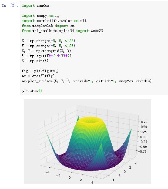
2.whats_new_99_mplot3d:
whats_new_99_mplot3d.py
import random
import numpy as np
import matplotlib.pyplot as plt
from matplotlib import cm
from mpl_toolkits.mplot3d import Axes3D
X = np.arange(-5, 5, 0.25)
Y = np.arange(-5, 5, 0.25)
X, Y = np.meshgrid(X, Y)
R = np.sqrt(X**2 + Y**2)
Z = np.sin(R)
fig = plt.figure()
ax = Axes3D(fig)
ax.plot_surface(X, Y, Z, rstride=1, cstride=1, cmap=cm.viridis)
plt.show()
同样执行 Cell,即可看到绘制出的图像。
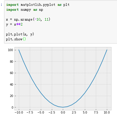
动手试试
最后,我们来尝试绘制一个二次函数图像,你可以自行实现,也可以参考下面代码:
import matplotlib.pyplot as plt
import numpy as np
x = np.arange(-10, 11)
y = x**2
plt.plot(x, y)
plt.show()
搭配 TensorFlow(可选)
TensorFlow™ 是一个采用数据流图,用于数值计算的开源软件库。它灵活的架构让你可以在多种平台上展开计算,例如台式计算机中的一个或多个CPU(或GPU),服务器,移动设备等等。
TensorFlow 最初由 Google 大脑小组的研究员和工程师们开发出来,用于机器学习和深度神经网络方面的研究,但这个系统的通用性使其也可广泛用于其他计算领域。
安装 TensorFlow
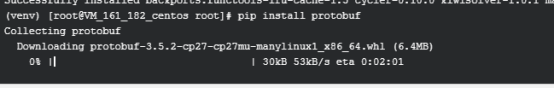
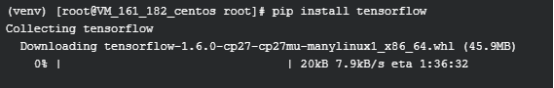
我们使用 pip 安装相关依赖及 Tensorflow
pip install protobuf
pip install tensorflow
测试 TensorFlow
关于 TensorFlow 的使用请移步其官网,这里只是测试其在 Jupiter 中是否可用。
点击这里打开 tensorflow.ipynb 编辑界面。
在 Cell 中加入以下代码(整理自官网 MNIST 教程):
示例代码:/tensorflow.py
from tensorflow.examples.tutorials.mnist import input_data
import tensorflow as tf
# The MNIST Data
mnist = input_data.read_data_sets("MNIST_data/", one_hot=True)
# Regression
x = tf.placeholder(tf.float32, [None, 784])
W = tf.Variable(tf.zeros([784, 10]))
b = tf.Variable(tf.zeros([10]))
y = tf.nn.softmax(tf.matmul(x, W) + b)
# Training
y_ = tf.placeholder(tf.float32, [None, 10])
cross_entropy = tf.reduce_mean(-tf.reduce_sum(y_ * tf.log(y), reduction_indices=[1]))
train_step = tf.train.GradientDescentOptimizer(0.05).minimize(cross_entropy)
sess = tf.InteractiveSession()
tf.global_variables_initializer().run()
for _ in range(1000):
batch_xs, batch_ys = mnist.train.next_batch(100)
sess.run(train_step, feed_dict={x: batch_xs, y_: batch_ys})
# Evaluating
correct_prediction = tf.equal(tf.argmax(y,1), tf.argmax(y_,1))
accuracy = tf.reduce_mean(tf.cast(correct_prediction, tf.float32))
print(sess.run(accuracy, feed_dict={x: mnist.test.images, y_: mnist.test.labels}))
按下 Shift + Enter,学习过程结束后可以看到输出了准确率(92% 左右)。
实验到此结束
本实验取自腾讯云实验室,是手工照着实验室内容做的
如今部分源可能存在过期问题,可以在云+问答中补充